In an attempt to explore and survey modern transfer learning techniques used in language understanding, researchers at Google AI introduced the T5 — Text-to-Text Transfer Transformer — which was proposed earlier this year in the paper “Exploring the Limits of Transfer Learning with a Unified Text-to-Text Transformer”. The T5 provides a unified framework that attempts to combine all language problems into a text-to-text format. Moreover, the authors have also open-sourced a new dataset called C4 — Colossal Clean Crawled Corpus — to facilitate their work.
Preface
It’s quite strenuous to make a significant stride in performance and surpassing the latest state-of-the-art benchmark when introducing a new ML model. Authors generally stack several performance boosters on top of each other in their papers in an attempt to overcome this challenge. They generally don’t want to report the changes to their algorithm without additional computation or dataset size, or they don’t have the resources to test this out anyways because training these large scale models like XLNet can be very expensive.
Researchers from Google AI took apart the many components of the transfer learning pipeline and natural language processing in this large-scale study. This includes comparing autoregressive language modelling, to BERT’s pre-training objective and XLNet’s shuffling objective. They further explored different ways of doing BERT’s MASS language modelling such as dropping spans rather than individual tokens. They also explore factors such as dataset size, the composition of the dataset and how to use extra computation. They take the learnings and scale it up to a 11 billion parameter model. This model is particularly amenable to transfer learning thanks to its text-to-text framework that allows developers to adapt this pre-trained model to their task. For instance, they could prefix it by asking a question, followed by the context or translating one spoken language to another.
This article will attempt to explain this paper that explores the limit of transfer learning and natural language processing from researchers at Google AI.
Introduction
The paper is a large-scale study on the different components of the pre-trained and fine-tuned NLP pipeline. The authors scale up their best found practices to a 11 billion parameter model with a very interesting text-to-text formulation of all natural language processing tasks. The authors tries to isolate these different factors of variation with the pre-trained and fine-tuned natural language processing pipeline. A lot of the previous mentioned papers have to combine different factors that will improve performance in order to get accepted into top conferences such as ICML and NeurIPS. For example, not only introducing a new pre-trained objective but also scaling up the model size or using a different way of cleaning the data or using a different dataset that is more in domain for the task that is going to be fine-tuned for the downstream performance evaluation.
Text-to-Text Framework
An interesting detail about this study is the text-to-text formulation of all NLP tasks. One such being the ‘Cola test’ (where you’re trying to determine whether a sentence is grammatically correct) the BERT model may be fine tuned for this by having a classification output on the CLS token index of the output layer of the BERT model.

Source: Google AI Blog — Exploring transfer learning with T5
But the T5 model is learning to take in text input and text output for all tasks. So in order to do translation, you see the model with the prefix “translate English to German” followed by what you want it to translate. Or the “cola sentence” for the glu/cola tasks of determining if the sentence is grammatically correct. This way of prefixing the task with natural language is really interesting way of thinking about the unified models that can do multi-task learning, pre-training on the same objective and then fine-tuned to many different tasks.
Factors of Variation Explored
The large scale study of the different factors of variation begins with the attention masking and foundational architecture for these pre-trained, self-supervised objectives. So the difference between the autoregressive language modelling or sequentially predicting the next token, compared to masked language modelling used in papers like BERT.
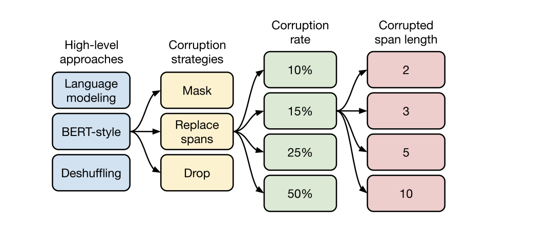
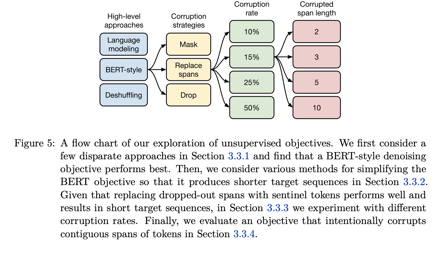
They further take apart the de-noising self supervised learning objective by replacing the spans and different ways of doing that using hyper parameters of corruption rate when the tokens were replaced by the mask, and the span length which we will get into later.
Then they look at the different architectures they can use. The encoder/decoder style model, the encoder only with shared parameters, LM, prefix LM etc. that affect the architecture of the transformer model that impacts the downstream performance.
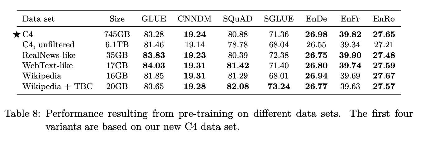
They also look at different datasets. The construct a new Colossal Clean Crawled Corpus (C4) that is inserted by doing just a web dump of all the text on the web. Originally around 6TB of data, that they clean into 750GB. They compare that clean C4 data with the Wikipedia dataset + Toronto book corpus or the web text style with the reddit filter (that was used in the GPT-2 paper).
They also take a look at the fine tuning strategies. How do you pre-train and fine tune on the tasks, how do you transfer all these different parameters to a new task, what stages of training on the supervised learning tasks and then fine-tune the unsupervised learning tasks, or training only on the unsupervised tasks and then fine tuning only on the supervised tasks.
Finally they talk about how to use extra computation to train these transformer models.
Value of Pre-Training
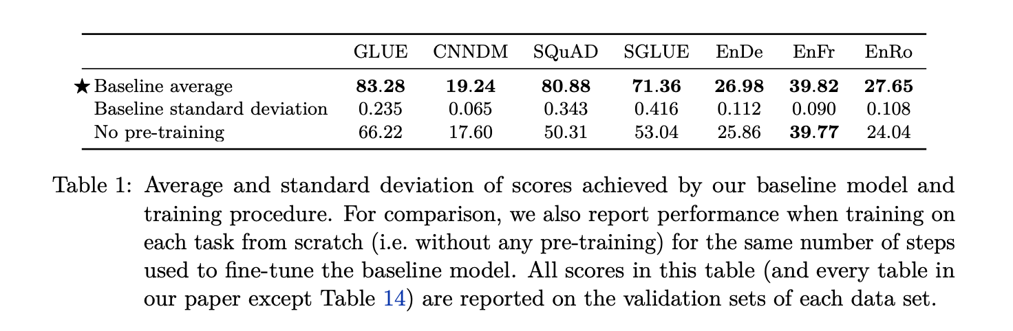
The first table shows the advantage of pre-training compared to randomly initialized model that’s fine tuned on the supervised learning task at hand. You can see the difference in the GLUE benchmark, CNN/Daily Mail summarization task, the SQuAD question and answer dataset. But you also see that there aren’t any gains in the translation tasks (English to German, French and Romanian respectively). This is attributed to their large datasets that do not benefit from the pre-training and fine tuning pipeline.
Attention Masking
Attention masking masking describes how much of the input the transformer is able to see when it’s producing the output.
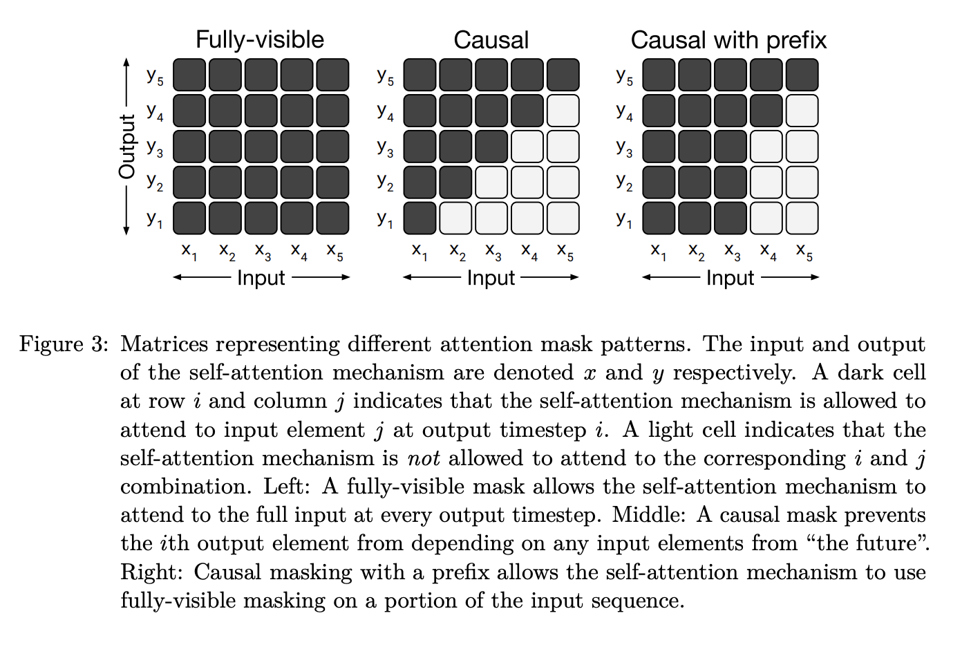
In the fully-visible setting, the transformer is able to see the entire input when its producing each token in the output. In the Causal setting, it sees token 1 as it is generating output 1 and the window slides over as it generates the sequence. Causal with prefix sees a portion of the initial sequence and then proceeds to behave like the Causal masking.
Corresponding Architectures
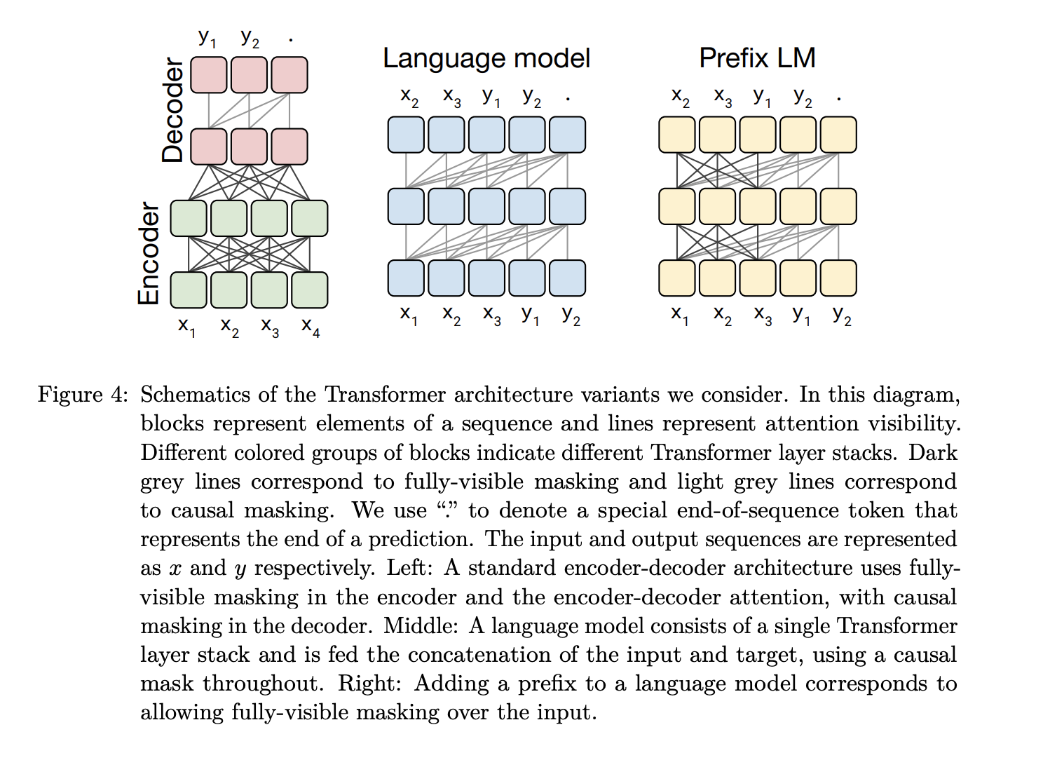
The Encoder-Decoder architecture corresponds to the fully-visible masking, where the entire input is visible while generating the output sequence.
The Language Model (LM) architecture is essentially the causal attention mechanism that was discussed earlier. It is an autoregressive modeling approach where you see x1 when generating x2, you see x1 x2 when generating x3 and so on.
The Prefix LM architecture is a mix of both the BERT-style and language model approaches. It avoids having to predict x1 x2 x3 by already seeing that in the prediction for y1 and then sliding over for y2 y3 and so on.
Architecture Performance Evaluation
Experiments showed that the Encoder-Decoder architecture obtained the best results.
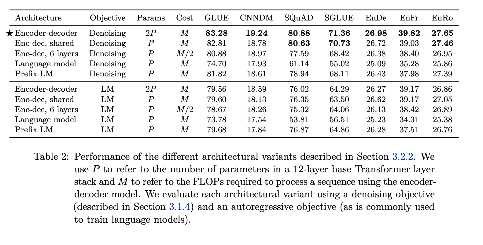
This table differentiates the different architectures using the denoising objective where you’re randomly corrupting the tokens and only predicting the corrupted tokens. Whereas the autoregressive objective (LM) involves autoregressively predicting the next token, sliding the window and predicting the next token and so on to pre-train the models.
The first two architectures are the encoder-decoder with the difference being the sharing of parameters. The third encoder-decoder model has 6 layers each in the encoder and decoder, as compared to the 12 layers in the original one. The language model (LM) and the prefix LM architecture are what we saw earlier in the masking techniques where varying degrees of the input are visible while generating the output token.
Denoising Objective
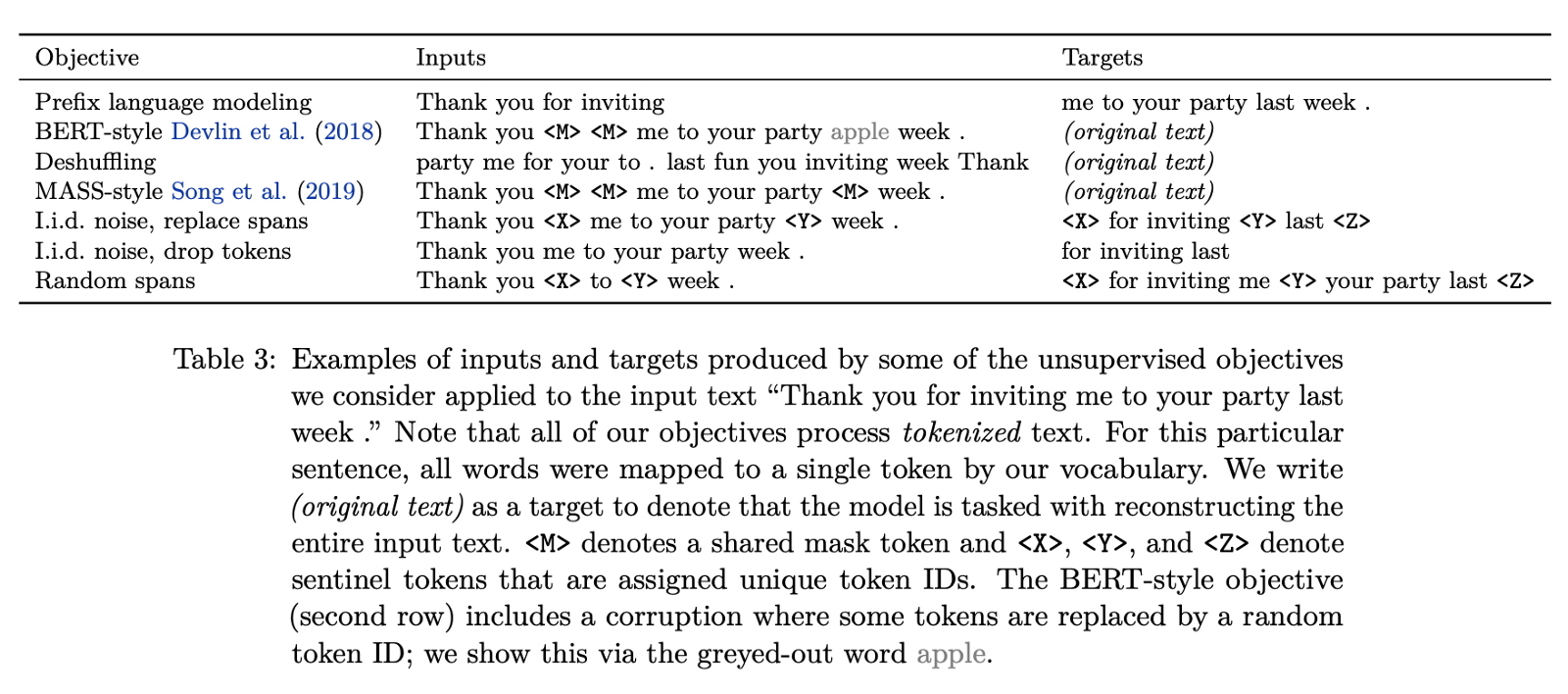
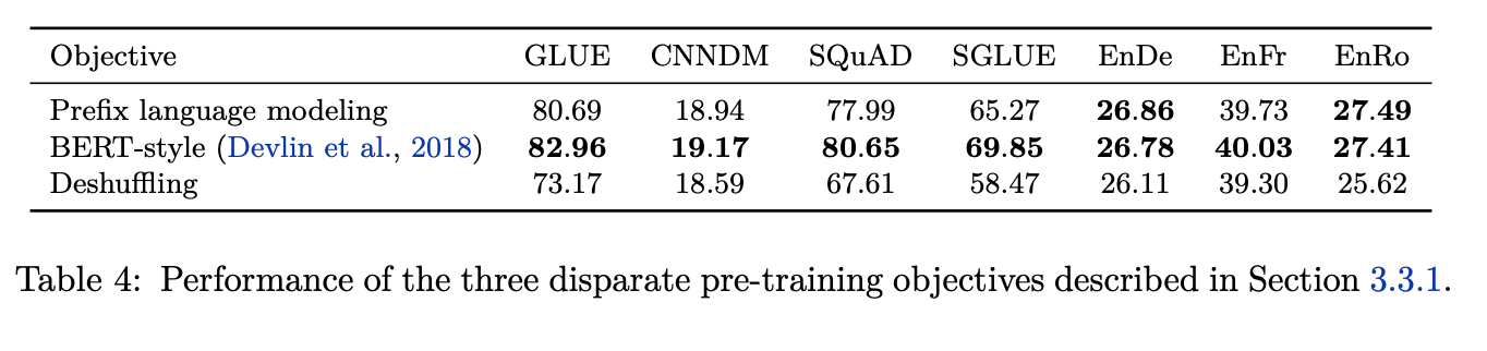
This table further explores the denoising self supervised objectives. The baseline is set without denoising using the prefix language modeling where you see an input ‘Thank you for inviting’ and predict the output target ‘me to your party last week’ by sliding over the window i.e.- you slide over the output token ‘me’ into the input while predicting ‘to’ and then slide over ‘to’ while predicting ‘your’ and so on.
The BERT-style model uses mask style modeling where you mask out certain intermediate tokens and predict the entire sequence again. You can also switch out words (in this case switching ‘last’ for ‘apple’) as a way of randomly corrupting the words and predicting the correct word.
Deshuffling (was introduced in XLNet) where you shuffle the sequence and then you reconstruct the sentence from this random order.
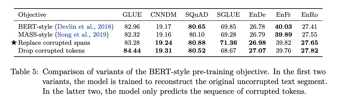
MASS-Style mask randomly introduces these to tokens through the input sequence and predict the entire sequence again.
Replacing spans involves randomly masking sequence of tokens. For instance, ‘for inviting’ is masked entirely and the length of the sequence is hidden under the
Drop tokens is similar to replacing spans but does not indicate the spans (
Span Corruption Strategy
They further compare the replace span and drop token strategy as a way of corrupting tokens in this mass language modelling task.

What they observe is that the replace span works well in some tasks whereas drop corrupted tokens works better on others. So it’s interesting to see the difference when you explicitly indicate the the location of the dropped token versus where you don’t indicate anything in the input regarding the spans of the tokens being dropped.
They also observed these pre-training efficiency gains from smaller output sequences. So in the original Table 3, the objectives involving predicting just the output tokens/spans of tokens (drop token) rather than the complete sentence (BERT-Style) had a much smaller encoder output and therefore a faster training.
Self-Supervised Learning
Between the Language Modelling technique where we slide over the input tokens to predict the output, the deshuffling technique of randomly rearranging the input tokens, the BERT-Style model (a.ka. denoising objective) of masking a sequence of words from the sentence and training the model to predict these masked words, seemed to perform the best.
As for the corruption strategies, they preferred replacing the spans over masking or dropping the tokens without indicating the token has been dropped in that index of the sentence.
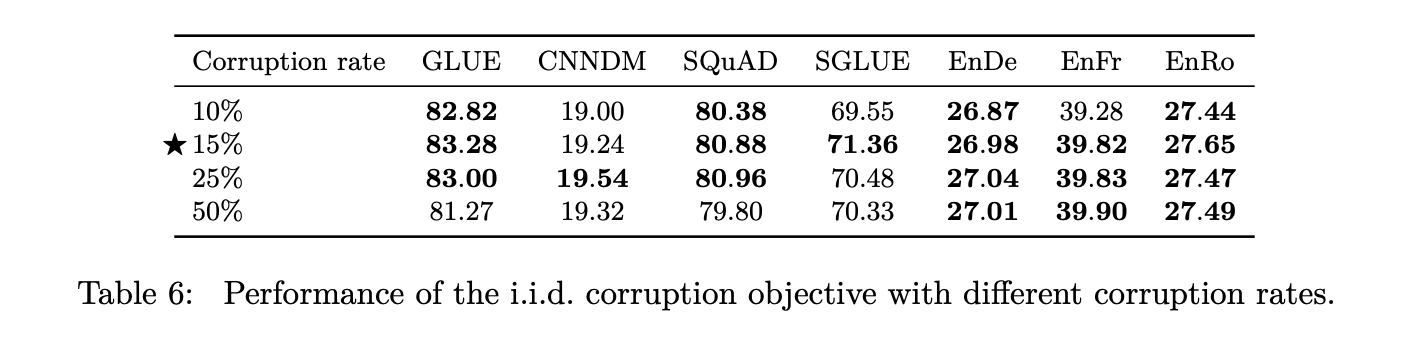
They also explored the hyper parameters of corruption rate and corrupted span length. The corruption rate is the probability that a token is going to be corrupted and replaced with
This is also seen in the following tables where the denoising objective performs the best under various tasks as compared to the other models. Comparing the corruption strategies also indicates how replacing spans works best in the majority of the tasks such as the SQuAD dataset, CNN/Daily Mail dataset and the SuperGLUE benchmark.
Datasets
The other factor of variation that this paper looks into is the dataset that is used in the pre-training self supervised learning objective.
They start off with the Colossal Clean Crawled Corpus (C4) which is obtained by scraping web pages and ignoring the markup from the HTML. However, Common Crawl contains large amounts of gibberish text like duplicate text, error messages and menus. Also, there is a great deal of useless text with respect to our tasks like offensive words, placeholder text, or source codes.
For C4, the authors took Common Crawl scrape from April 2019 and applied some cleansing filters on it:
- Pages with placeholder texts such as ‘lorem ipsum’ are removed.
- “JavaScript must be enabled” type warnings are removed by filtering out any line that contains the word JavaScript.
- For removing duplicates, three-sentence spans are considered. Any duplicate occurrences of the same 3 sentences are filtered out.
- Source codes are removed by removing any pages that contain a curly brace “{” (since curly braces appear in many well-known programming languages).
- Removing any page containing offensive words that appear on the “List of Dirty, Naughty, Obscene or Otherwise Bad Words”.
- Retaining sentences that end only with a valid terminal punctuation mark (a period, exclamation mark, question mark, or end quotation mark).
- Finally, since the downstream tasks are mostly for English language, langdetect is used to filter out any pages that are not classified as English with a probability of at least 0.99.
This resulted in a 750GB dataset which is not just reasonably larger than the most pre-training datasets but also contains a relatively very clean text.
They also use the RealNews-like dataset which contains new articles. WebText-like dataset that uses a reddit filter (used in the GTP-2 paper) where an article is included only if there is a corresponding reddit post with atleast 3 upvotes on it.
Dataset Size
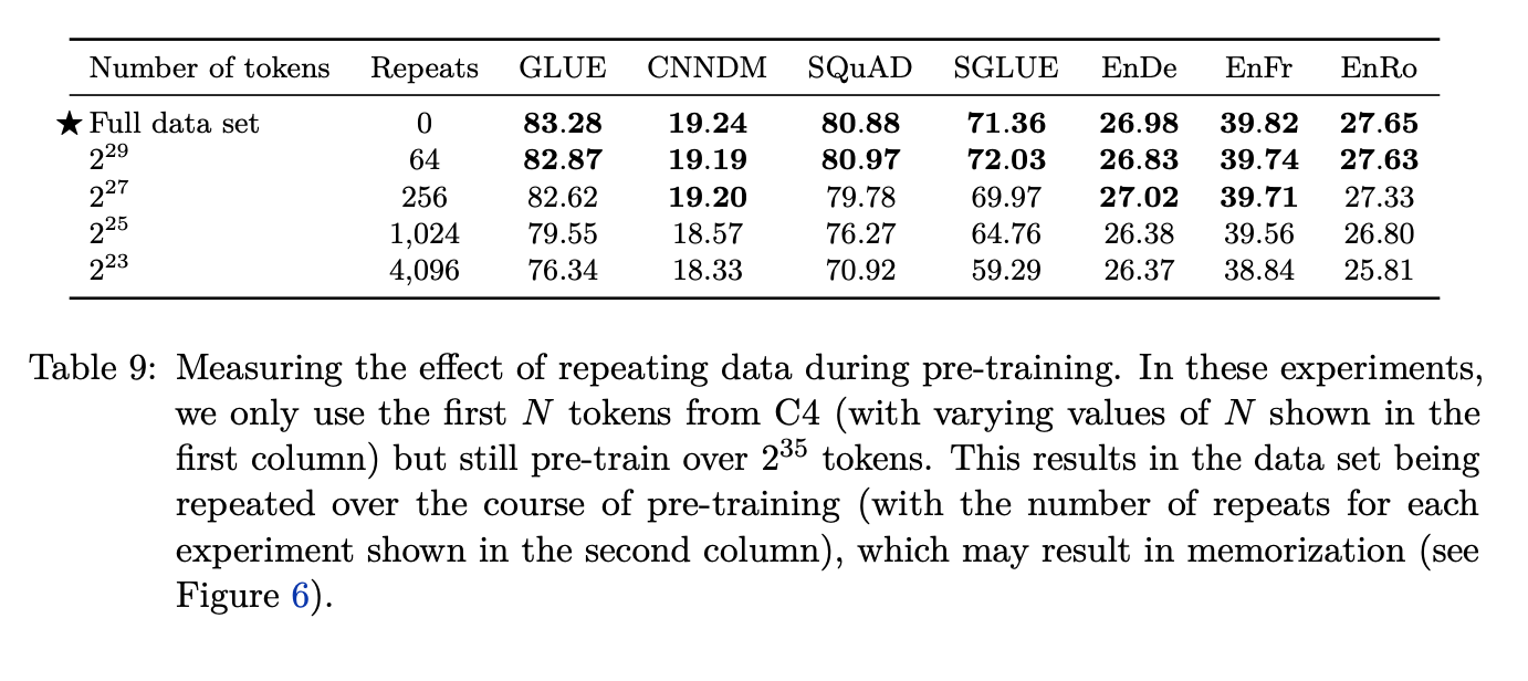
They also explore the dataset size by downsampling their C4 dataset into various subsets to show when overfitting happens with respect to the size of the down sampled dataset. They also indicate how many times these different subsets of the data involve repeating the same token as it is passed in mini batches for pre-training objective.
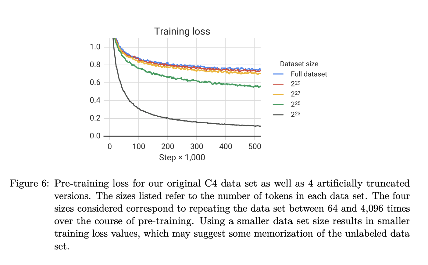
A dramatic overfitting happens for the 2²³ dataset and a similar trend with the other versions of the dataset, but no visible overfitting with the full dataset.
Fine Tuning Strategy
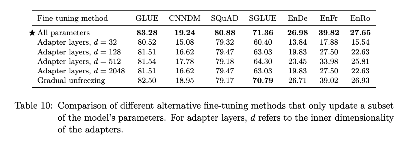
The authors study the strategy for fine tuning these models on down stream tasks such as question answering or natural language inference after they have been pre-trained on the BERT, replaced span self-supervised learning task on the C4 dataset.
The first way is to fine tune all the parameters, which is the most computationally challenging way of doing this where you pass the values through every single parameter of the original model that was fine-tuned on the self supervised learning task.
The other strategy is to use adapter layers, which are these intermediate layers of feed-forward normalization that help adapt the model to the new task without introducing too many parameters. So you still freeze all the original parameters from the self supervised learning training, but now you’re introducing these new layers that can corrupt these features in a way that it can do this new task.
There is also gradual unfreezing where you progressively unfreeze the layers of the transformer. For instance, layer 12 of the encoder and layer 12 of the decoder are being trained, then layer 11, 10, 9.. and so on as you continue the training.
As per the findings, they conclude that fine tuning all parameters works best despite it being the most computationally expensive.
Task Imbalance
Next they explore strategies for including supervised learning data with the unlabelled data in the pre-training objective.
One of the really interesting characteristics of this text-to-text framework is that it’s really easy to mix this supervised learning data with the self-supervised learning data because it has the similar framework of just passing it in with the prefix that denotes the task that it’s performing with supervised learning or some way of doing the unsupervised learning.
But they find that there is this issue of task imbalance. We know that there are these different tasks such as cola, sentiment analysis, etc. and along with that are different dataset sizes. We need different ways of balancing out the sampling the mini-batches with respect to pre-training the model if you’re going to try the multi-task training. It seems intuitively like this would obviously be better than only using the unlabelled data, they don’t really realize these gains quite yet.
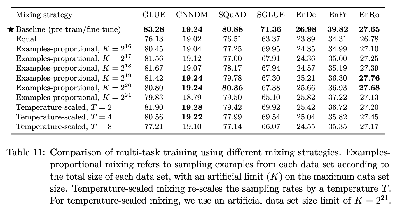
They find that the baseline study of pre-training on the unlabelled data and fine tuning into the label task works better than trying to integrate the supervised learning data in the pre-training objective.
The following table further shows the results of this study.
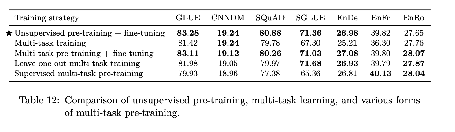
The first strategy is of pre-training on the unsupervised data and then fine-tuning on the supervised learning. The second one — multitask training- is something we saw earlier where instead of doing fine-tuning, you’re only pre-training on the different tasks and thats just the final model that is going to be used for evaluation. The third one involves fine-tuning on the individual tasks. So you do multi-task learning on sentiment analysis, question-answering, etc. and then fine-tune it to the particular test its going to be evaluated on such as GLUE, CNNDM, etc.
Leave-one-out is where you leave out the task that’s going to be fine-tuned in the pre training. So if its going to be evaluated with the SQuAD benchmark, you leave out the SQuAD dataset in the pre-training and then only see those training samples in the fine-tuning.
Supervised multi-task pre-training describes not using the unsupervised objective at all and just doing the multitask pre-training and then using it for these different benchmarks.
Extra Computation
The next question the authors look at is how to use extra computation with pre-training these transformer language models.
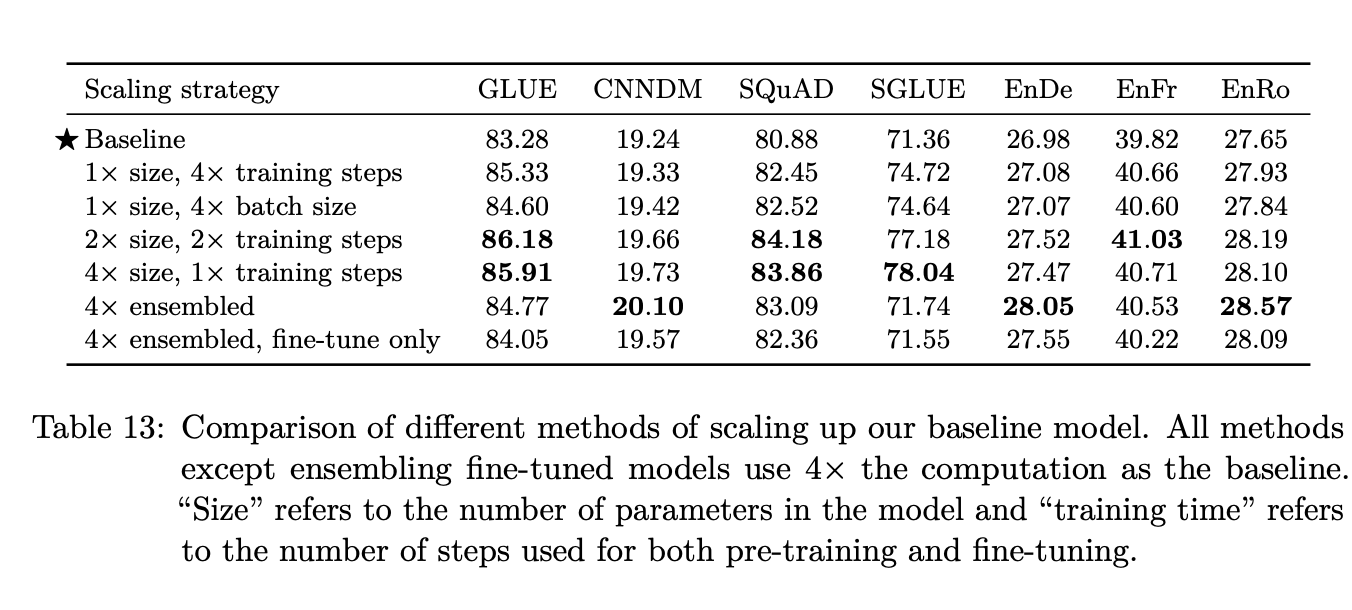
They first explore by increasing the training steps and then increasing the batch size which doesn’t perform as well. They also try increasing the size of the model and doubling the training steps, increasing the size and keeping the same number of training steps. They also compare this with certain ensemble methods.
Interestingly, they find that the four times in the size and not increasing the training steps at all has the best performance. Whereas you might expect that a bigger model, with the same amount of training time, might not have enough time to fit the data.
But this is inline with a certain recent study that suggest the best way of doing this is to train a large model and stop training early, and then heavily compress them all for the sake of efficiency.
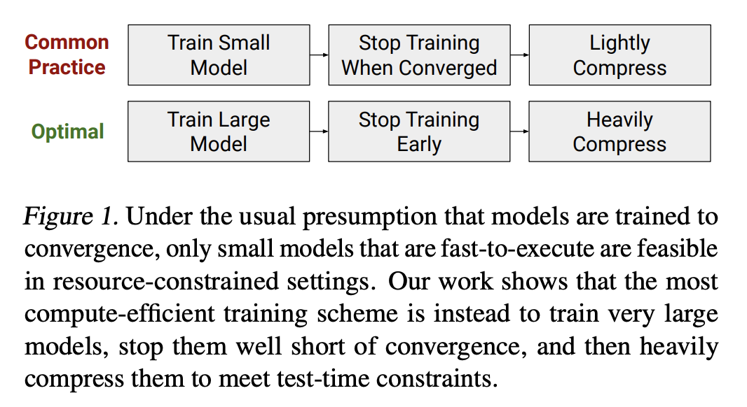
Source: Train Large, Then Compress
Larger models are significantly more sample-efficient, such that optimally compute-efficient training involves training very large models on a relatively modest amount of data and stopping significantly before convergence. — “Scaling Laws for Neural Language Models” abstract
Ensembling
Ensembling is an interesting technique technique that involves having the same model architectures, but you train each one with different original random parameters that result in different predictions from the model. You would then average out the predictions of the model.
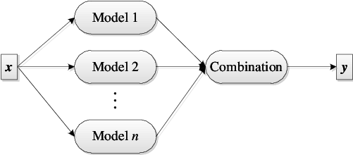
There are other ways of ensembling like having a different architecture, different ordering of the batches or entirely different pre-training objectives.
Scaling up
The authors then then take all the findings from this study — the self supervised learning objective, the C4 dataset — and then scaling up the model size to 3 billion and 11 billion parameters.
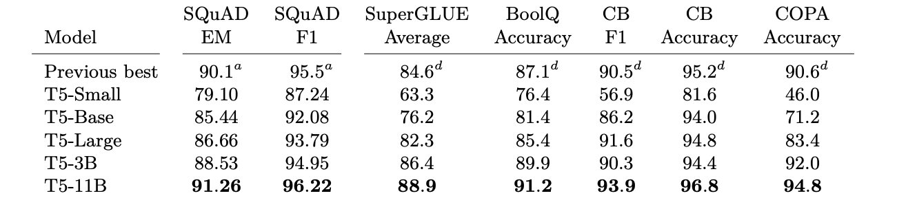
You notice these major gains in the Stanford Question-Answer dataset compared to the base model (T5-Base).
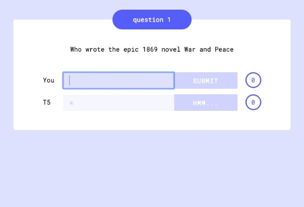
Applications
In the Google AI blogpost, the authors show the performance of the T5 model with 11 billion parameters on this trivia Q&A where it tries to answer all these different questions just from memory.
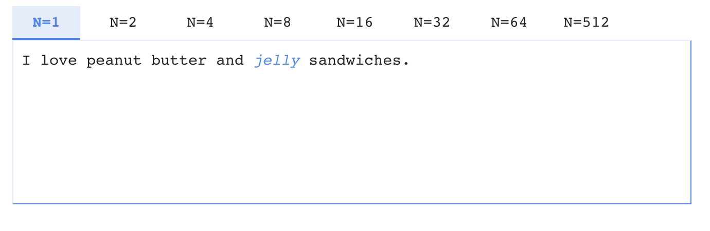
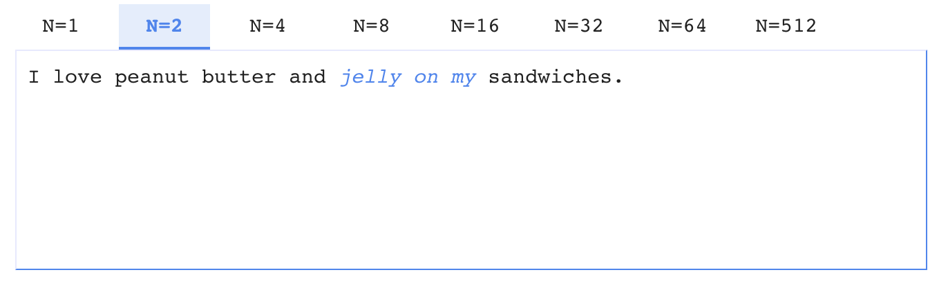
They also introduced this “Fill-in-the-Blank Text Generation” tool (available on the blog) where there is this sentence and you have to select the number of words to fill in. With each selection of N (number of words) there are different variations of a logical sentence being created.