
This article aims to explore an efficient transformer model from Google AI called the Reformer, which was proposed earlier this year in the paper “Reformer: The Efficient Transformer”. To overcome the efficiency related short-comings of the standard transformer, the reformer presents a way to approximate full attention and attention over long sequences. It also proposes ideas of reducing the memory requirements of training transformer models. This results in a model that is capable of handling a context window of upto a million words on a single GPU with 16GB of memory, and yet accuracy at par with the Transformer model.
Preface
When it comes to understanding sequential data such as natural language, music or videos, there is a major dependency on long term memory to build credible context. In a way, the feed-forward neural network provided us with a solution by taking the first few tokens as an input to generate the next logical output token, but severely lacked in context mapping over large sequences. To tackle this, the idea of Recurrent Neural Networks (RNN) came along that generalised the idea of the feed-forward neural network, but with an “internal memory” to improve this long term dependency. But RNNs still struggled with training long sequences due to the gradient vanishing and exploding problem which made it harder to remember past data in the memory. To resolve this issue, Long Short Term Memory (LSTM) was implemented, which is essentially a modification of RNNs by introducing back propagation and gating techniques to pick and choose what to remember and what to forget at each stage of the training process.
In a similar evolution, the Transformer model was introduced to overcome the severe performance bottleneck of RNNs as it processed the input sequences sequentially. You see, GPUs are designed and optimised to process information in parallel. And therefore, it only made sense that the model architecture conformed to this flow to make the most out of the hardware. At its core, it uses the concept of “attention” as a way of focusing on just the tokens relevant to the word being predicted and does away with the sequential flow of data. Currently, transformers such as the T5 text-to-text transformer generate state of the art results.
But where the transformer excels in performance, it has its shortfalls in terms of efficiency.
Efficiency Shortcomings of Transformers
- Attention Computation: Given a sequence of length L, the computational and space complexity of a transformer is O(L²). So for large sequence such as 64K or above, it would clearly struggle.
- Large Number of Layers: The size of the transformer model is a direct function of the number of layers. Which means that a transformer model with N layers would consume N-times the memory than a single layer model. This is because the activation for each layer needs to be stored for back-propagation.
- Depth of Feed-forward Layers: The depth of the feed-forward layers are usually much larger than the attention activation layers and hence takes up large memory storage.
To tackle each of these issues, the Reformer model adopts two techniques within the architecture: locality-sensitive-hashing (LSH) to reduce the complexity of attending over long sequences, and reversible residual layers to more efficiently use the memory available.
Locality Sensitive Hashing (LSH) Attention
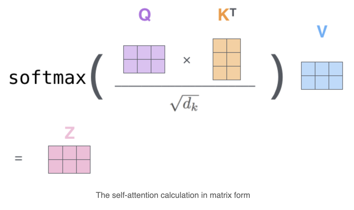
In the original Transformer model, we calculated the attention by first activating the actual embeddings with 3 different vectors — Query(Q), Key(K) and Value(V) — for each token. Then using the following dot product formula, we calculate the attention, which basically tells us how much each vector contributes to obtaining a given vector.
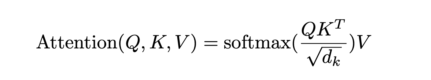
If you observe closely, the QKT is basically a matrix multiplication that results in a computational and memory cost O(L²) (given that the shape is [L, L]) which is a big bottleneck and quite inefficient.
To resolve this, the authors first suggest to use the same weights for both the Query(Q) and Key(K). Unlike the original transformer, where Q, K and V are calculated using 3 different set of weights. According to the paper, this sharing of weights — known as the shared QK-model — does not affect the performance of the transformer, but would save memory space in storing two separate sets.
Also the calculation and storage of the full matrix QKT seems quite unnecessary. We are only interesting the softmax(QKT) which helps the largest elements dominate in a typically sparse matrix. Therefore for every query (q) in the matrix Q, we need to find a set of keys (k) that are closest to q. For instance, if K is of length 64K, for each q we would only consider a subset of 32 or 64 close keys. Therefore this attention would find the nearest neighbour keys of the query quite inefficiently.
The authors identify this and use the search logic of nearest neighbours to replace the dot product attention with locality-sensitive hashing (LSH) and hence change the complexity from O(L²) to O(L log L).
Locality Sensitive Hashing (LSH)
The LSH algorithm helps approximate the nearest neighbours in a high dimension space quite efficiently. To understand this better, imagine 2 points in a 2 dimensional space. The idea of similarity in this space is synonymous with the distance between the two points. The same idea can be visualised for 2 points in 3 dimensions too. But this gets complicated quite quickly when the number of dimensions increase.
In a transformer, we map the each of the tokens to a vector space where the vector representations for all the tokens in the vocabulary co-exist. The vector representation is such that during training, the model is aware when two or more words are similar because of how close their vectors are (and conversely how dissimilar the words are based on how far the vectors are spaced).
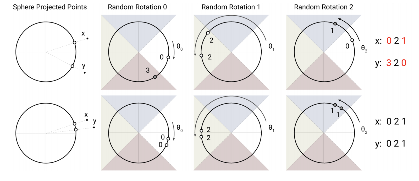
Now imagine 2 points(x and y) in the vector space that lie on a circle/sphere. This circle is equally divided into 4 zones, each with its own distinct code. We rotate this circle randomly thrice (this depends on the length of the hash, in this case hash length is 3). There are two cases (top and bottom row) illustrated in the figure above:
- Points x and y are spaced far apart in the first (top) case. During random rotations, the probability that both the points land in the same hash zone is low. For instance in rotation 0, point x lands in the hash zone with value 0 and y lands on the hash zone with value 3. But in rotation 1, they both land on the same hash zone i.e. — hash zone 2.
- Points x and y are spaced close together in the second (bottom) case. Therefore during random rotations, the probability that both points land in the same hash zone is high. You see that in each of the 3 random rotations, both points have ended up in the same hash zone and hence resulted in having the same hash values of 021.
This clearly shows that similar points will have a high probability of having the same hash value.
LSH Attention
The traditional transformer calculates the attention for each query separately, which is a sequential task in a parallel architecture leading to a bottleneck. What if instead of performing the complete calculation, we find a way to determine an approximate set of keys closest to the given query and compute the attention only for this relatively tiny set without compromising on performance? Well thats exactly how LSH attention works!
Therefore instead of calculating attention over all of the vectors in Q and K matrices, we do the following:
- Find the LSH hashes of the Q and K matrices.
- Compute standard attention only for the k and q vectors within the same hash buckets.
To increase the probability that similar items do not fall in different buckets, we perform the steps 1 and 2 multiple times and this is called multi-round LSH attention.
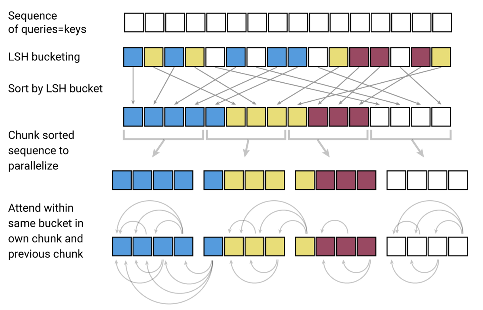
According to the paper, the above diagram illustrates the LSH mechanism in the Reformer.
- The sequence of queries and keys are assigned to their various hash buckets (each bucket for each value, shown here with different colours) using the LSH algorithm we discussed earlier.
- We sort the query/key vectors based on the LSH bucket.
- We need to chunk the sequence to help parallelise. Therefore we need to divide the sequence into batches. It’s not possible to equally divide the sequence as the hash bucket sizes vary, hence we define a single batch size with an offset of 1.
- We calculate the attention for the vectors from the same bucket and same chunk and one chunk back.
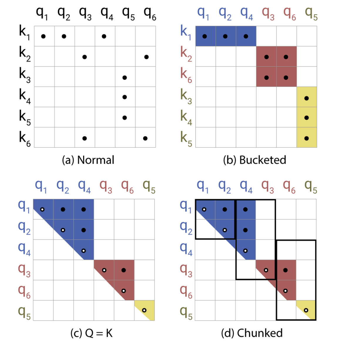
The Attention matrices shown above depict the varieties of attention at each step. In (a) the attention is quite sparse, but is not taken advantage of. In (b) the queries and keys have been sorted according to their hash bucket. Matrix (c) shows the sorted attention matrix where pairs from the same bucket are clustering near the diagonal. Finally figure (d) follows the batching approach where chunks of m consecutive queries attend to each other, and one chunk back.
Reversible Transformer
To solve the second problem of large number of encoder and decoder layers, we introduce the idea of reversible residual network (RevNet).
Reversible Residual Network (RevNet)
Each sub-layer (attention and feed-forward) of the transformer in both the encoder and decoder is wrapped in a residual layer. This layer is essentially a layer normalization and addition between the input and output of each of the sub-layers. They are also known as Residual Networks (ResNets) and have proven to be very effective in dealing with the vanishing gradient problem in deep neural networks. The problem is we need to store the activation values of each layer in the memory to calculate the gradients during back-propagation. This is a major bottleneck in memory consumption as more the number of layers, more the memory is needed to store them.
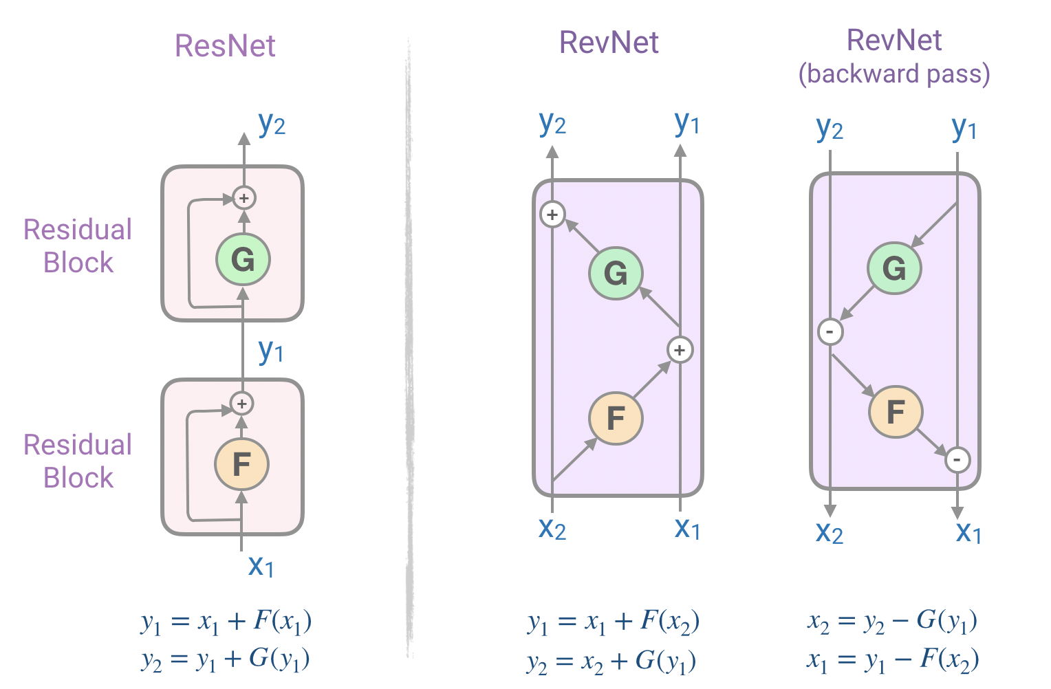
To tackle this problem, we make use of the reversible residual network (RevNet) which has a series of reversible blocks. In RevNet, each layer’s activations can be reconstructed exactly from the subsequent layer’s activations, which enables us to perform back propagation without storing the activations in memory. In the above figure, we can calculate the inputs x1 and x2 from the blocks output y1 and y2.
RevNet Transformer
In the above figure, if we replaced the functions F and G with the attention and feed-forward layers inside the RevNet block, we get:
Y₁ = X₁ + Attention(X₂)
Y₂ = X₂ + FeedForward(Y₁)
We are able to store the activation values only once instead of N times, as compared to the standard residuals and hence save a lot of memory essentially making this arrangement a reversible transformer.
Chunking
To tackle the third and final problem with transformers where the number of layers in the feed-forward layer is much higher than the attention activation layer itself, we implement chunking.
Take for instance a sequence with 64K tokens. In a standard transformer, all outputs are calculated in parallel and hence the weights take more memory. But since the computation in a feed-forward network are independent across position of the sequence, the computations for the forward and backward passes as well as the reverse computation can be all split into chunks. Hence the Reformer suggests to process this layer in chucks of ‘c’ as shown below:

We can therefore have the layer-input memory of a Reformer model independent of the number of layers by implementing both reversible layers (RevNets) and chunking.
Results
As per the paper, the authors conducted experiments on two tasks:
- imagenet64: an image generation task with sequences of length 12K
- enwik8: a text task with sequences of length 64K
Using these two tasks, they compared the effects and changes — reversible transformer and LSH hashing — to the traditional transformer in terms of this efficiency, accuracy and speed.
The following graphs shows the effects of two changes proposed by the authors.
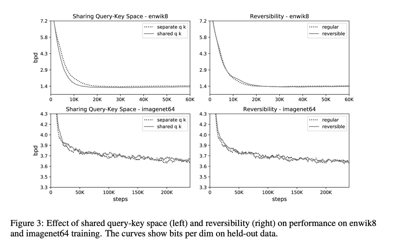
On the left hand side, we observe the accuracy graphs between the shared and separate QK attention models. Clearly, we are not sacrificing accuracy by shifting to the shared-QK model. In fact, for enwik8, it seems to train slightly faster.
On the right hand side, we see that the reversible Transformer saves memory without sacrificing accuracy in both tasks.
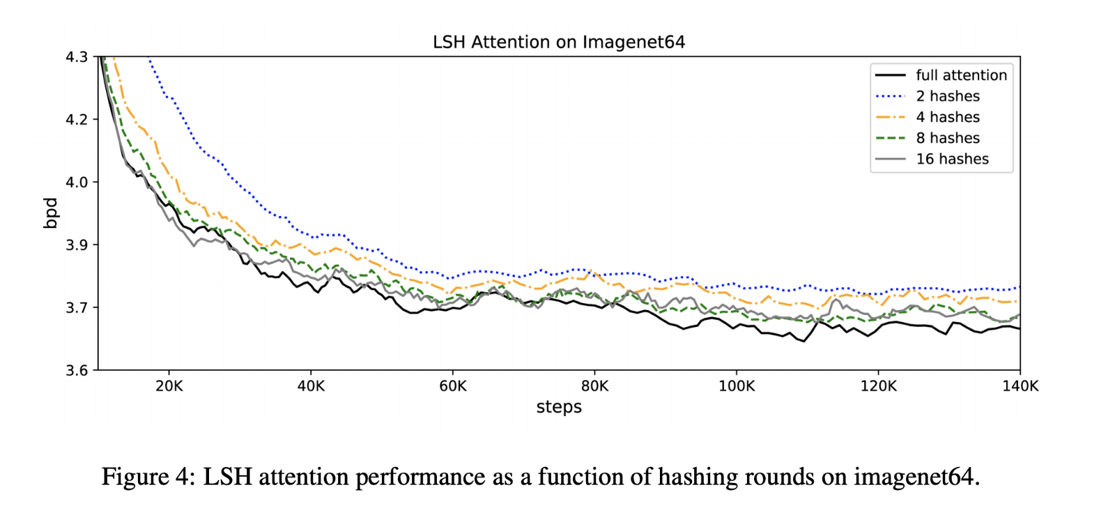
When it comes to the LSH attention, which is an approximation of the full attention, its accuracy improves as the hash value increases. In fact the model performs comparably when trained for 100K steps.
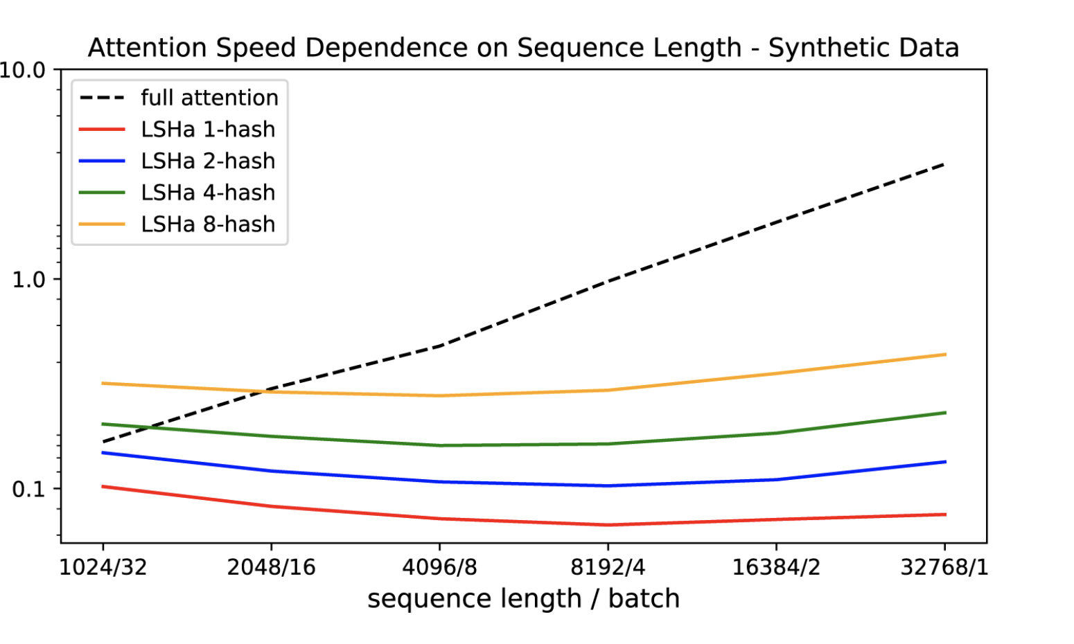
The experiments also demonstrate that the conventional attention slows down as the sequence length increases, while LSH attention speed remains steady.
The final Reformer model performed similarly compared to the Transformer model, but showed higher storage efficiency and faster speed on long sequences. — The Paper
Application
The Reformer has shown to work well in the space of large-context data such as image generation. The authors decided to perform an experiment using the Imagenet64 dataset.
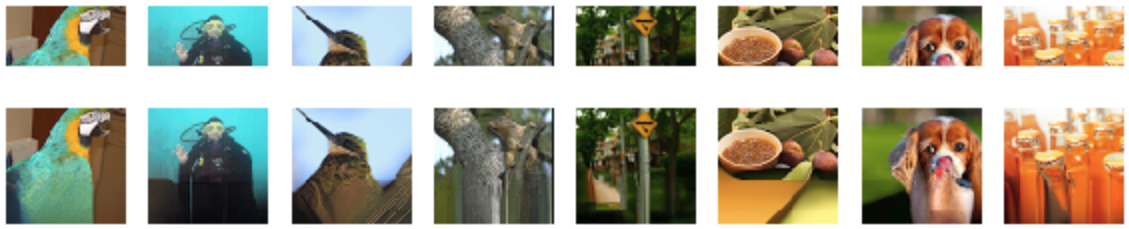
Starting with the images in the top row, the Reformer generates the results shown in the corresponding bottom row.
Similarly impressive results have also been seen in generation of text data where the model is able to generate an entire novel on a single device (Check out this colab notebook to try it out).