
This is the second article in a multi-part series to explore and understand the research done in developing language models to help debunk false information available in the public domain. There are many aspects of this system and I have separated them into multiple parts, each highlighting a particular research work that inspired me.
In the previous article, we took the example of the FEVER dataset to understand the process involved in creating a dataset from scratch. The claims were labelled under one of three categories - SUPPORTED, REFUTED and NOTENOUGHINFO to indicate the veracity of the claim. We also discussed the three ways in which the dataset was used to validate against its label. FEVER is one of many claims datasets that are used today to accurately predict and classify false information.
Another such dataset is the MultiFC dataset that takes a more novel approach. It collects its claims from 26 different fact checking websites, paired with textual sources and rich metadata and labelled by experts. As a result, we get a dataset that is much larger and more importantly, associates to the real-world much better. Further analysis is done to identify entities mentioned in the claim.
What I’d like to focus on in this article is the approach taken to train a veracity model with the help of this dataset. Also we’ll take a look at the cases where adding evidence pages and/or metadata improving the performance of the model or not. We’ll also take a look at a model that jointly ranks evidence pages and performs veracity prediction.
Note that the following article is my interpretation of the original work done by the authors and creators of MultiFC. I have selected a subset of the white paper to help highlight the model design process in this specific domain.
Dataset Construction
The authors train and compare multiple different models by focusing on two primary approaches - by considering only the claims and/or also encoding the evidence pages as well. Evidence pages are retrieved by sending the claim to the Google Search API verbatim and scrapping data from the top 10 resulting web pages. A certain level of preprocessing takes place to overcome roadblocks such as SSL/TLS protocol, Timeout, URLs to PDFs rather than HTML, etc. Also to better understand what the claims are about, entity linking takes place for each claim. Entity linking is done to connect mentions of named entities such as people, places, organisation, etc to the claim through their respective Wikipedia pages. Different entities with the same claim are disambiguated. This results in 42% of the claims having entities linked to Wikipedia pages. We will later see how these entities are used as part of the metadata to improve performance. The authors list the top 30 most frequenting entities:
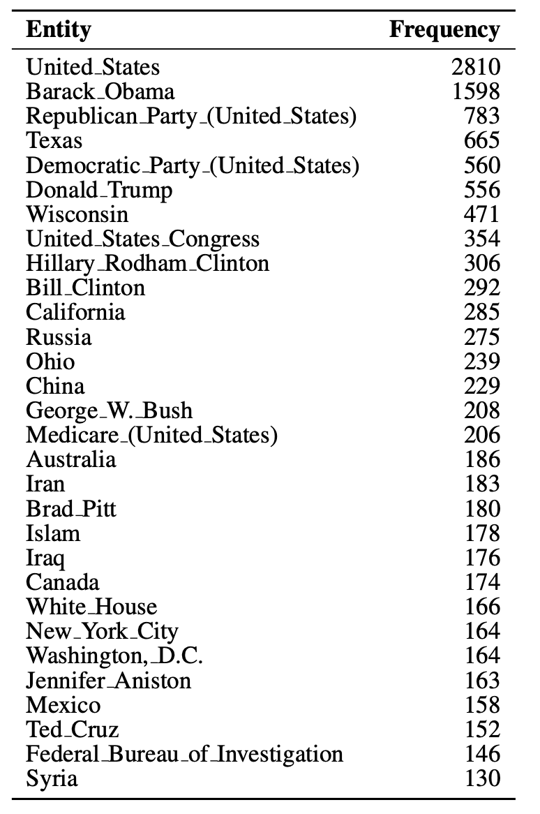
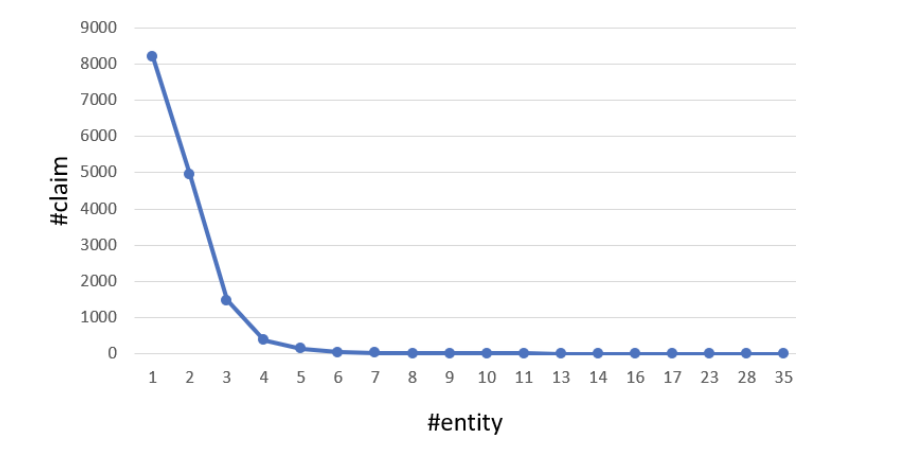
Another interesting observation the authors make are the majority of the claims have one to four entities, with the highest number of entities of 35 occurring in only one claim. In the top 30 most frequenting entities, ‘United States’ is the most frequented. This makes sense as most fact checking websites are US based.
Now that we have all the data, let’s start by first training a model on the claims alone.
Multi-Domain Claim Veracity Prediction with Disparate Label Spaces
Different websites use different labels, which makes training a claim veracity prediction model complicated. One way to solve this is to map the labels of one source to another. But there are no clear guidelines to perform the mapping process. Also given the large number of labels, it’s not very feasible. The other approach the authors take is to learn how these labels relate to one another as part of the claim veracity model. They do this using the multi-task learning (MLT) approach (which is inspired by collaborative filtering) which is know to perform well in pair wise sequence classification tasks with disparate label spaces. This was done by modelling each domain on it own task in a MLT architecture and the labels are projected on a fixed-length embedded space. Predictions are then made by taking the dot product between the label embeddings and the claim-evidence embeddings. This allows the model to understand the semantics between how close the labels are to each other.
To define this formally, the authors frame the problem as a multi-task learning one. Given a labelled dataset, we imagine T tasks (\(\tau_1,...,\tau_T\)) is provided at training time with target task \(\tau_T\) is of particular interest. The training dataset for task \(\tau_i\) consists of N examples \(X_{\tau_i}=\{x_1^{\tau_i},...x_N^{\tau_i}\}\) and their labels \(Y_{\tau_i}=\{y_1^{\tau_i},...y_N^{\tau_i}\}\).
The base MLT model shares its parameters across tasks and has a task-specific softmax output layers that output a probability distribution \(p^{\tau_i}\) for task \(\tau_i\) as: \(p^{\tau_i} = softmax(\textbf{W}^{\tau_i}\textbf{h}+\textbf{b}^{\tau_i})\) where softmax is defined as \(softmax(x)=\dfrac{e^x}{\sum_{i=1}^{||x||}e^{x_i}}\), weight matrix is given by \(\textbf{W}^{\tau_i} \in \mathbb{R}^{L_i \times h}\) and bias term defined as \(\textbf{b}^{\tau_i} \in \mathbb{R}^{L_i}\) for the output layer of the task \(\tau_i\) respectively. Also \(\textbf{h} \in \mathbb{R}^h\) is the joined learned (as the weights are shared) hidden representation, \(L_i\) is the number of labels for tasks \(\tau_i\) and \(h\) is the dimensionality of h.
Label Embedding Layer
As mentioned before, we need to find the semantic of one label to another. This is done by mapping the labels of all tasks on a joint Euclidian space called a Label Embedding Layer (LEL). Unlike before where we trained separate softmax layers, a label compatibility function is used to measure how similar a label with embedding \(\textbf{l}\) is to the hidden representation \(\textbf{h}\) using the formula \(c(\textbf{l},\textbf{h}) = \textbf{l} \cdot \textbf{h}\) where \(\cdot\) is the dot product. To make sure \(\textbf{l}\) and \(\textbf{h}\) have the same dimensionality, padding is applied.
For the prediction, matrix multiplication and softmax are used in the formula \(\textbf{p} = softmax(\textbf{Lh})\) where \(\textbf{L} \in \mathbb{R}^{(\sum_iL_i)\times l}\) is the label embedding matrix for all tasks and \(l\) is dimensionality of the label embeddings.
When making predictions for individual domains/tasks, both at training and at test time, as well as when calculating the loss, a mask is applied such that the valid and invalid labels for that task are restricted to the set of known task labels. Here, the authors apply a task-specific mask to \(\textbf{L}\) in order to obtain a task-specific probability distribution \(p^{\tau_i}\) . Since the LEL is shared across all tasks, this allows the model to learn the relationships between the labels in the joint embedding space.
Joint Evidence Ranking and Claim Veracity Prediction
As part of the baseline, we only considered the claims in the previous model. This model ignores the evidence supporting or refuting our claim, hence we end up guessing the veracity on the stylometric differences observed in the claim text.
Therefore, the authors introduce another type of model that encodes 10 pieces of evidence along with the claim. Note that the authors have decided to include search snippets of the evidence rather than complete webpages. This is due to the challenges such as encoding large pages, parsing elements such as tables and PDF files, images and videos. This could be potential future work to improve the quality of evidence. In this case, the search snippets work pretty well as they already contain summaries of the part of the page related to the claims.
We define this formally by obtaining N examples \(X_{\tau_i}=\{x_1,...,x_N\}\). Each example consists of claim \(a_i\) and \(k=10\) evidence pages \(E_k = \{e_{1_0},...,e_{N_{10}}\}\). BiLSTM is used to encode the claim and evidence to obtain a sentence embedding. We also want to combine claims and evidence into sentence embeddings into joint instance representations. We use a model variant called the crawled_avg which is the mean average of the BiLSTM sentence embeddings of all evidence pages (signified by the over line) and concatenate those with the claim embeddings.
\[s_{g_i}=[\textbf{h}_{a_i};\overline{\textbf{h}_{E_i}}]\]Here, \(s_{g_i}\) is the resulting encoding for training example \(i\) and \([\cdot;\cdot]\) signifies vector concatenation. But the disadvantage is that all evidence in this case will be given equal weightage.
Evidence Ranking
Unlike crawled_avg, the authors define a new model called crawled_ranked that learns the compatibility between the instance claim and each evidence page. It ranks evidence pages by their utility for the veracity prediction task, and then uses the resulting ranking to obtain a weighted combination of all claim-evidence pairs. No direct labels are available to learn the ranking of individual documents, only for the veracity of the associated claim, so the model has to learn evidence ranks implicitly.
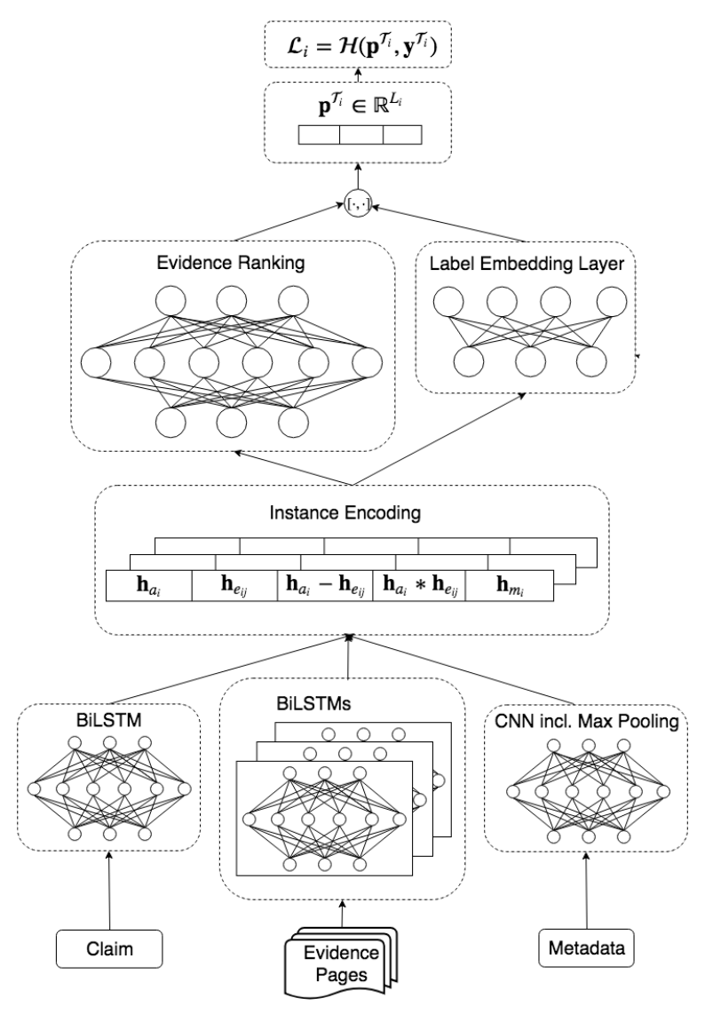
The claim and evidence representation is combined using the matching model using in natural language inference and adapted to combine the representation of each claim to its evidence.
\[s_{r_{i_j}}=[\textbf{h}_{a_i};\textbf{h}_{e_{i_j}};\textbf{h}_{a_i}-\textbf{h}_{e_{i_j}};\textbf{h}_{a_i}\cdot\textbf{h}_{e_{i_j}}]\]where \(s_{r_{i_j}}\) is the resulting encoding for training example \(i\) and evidence page \(j\) , \([\cdot;\cdot]\) denotes vector concatenation, and \(\cdot\) denotes the dot product.
The joint claim-evidence representation \(s_{r_{i_0}},...,s_{r_{i_{10}}}\) are projected onto a binary space via a fully connected layer (FC) followed by a non-linear activation function \(f\) to obtain a soft-ranking of claim-evidence pairs, of a 10-dimensional vector as
\[\textbf{o}_i=[f(FC(s_{r_{i_0}});...;f(FC(s_{r_{i_{10}}}))]\]where \([\cdot;\cdot]\) denotes concatenation.
Final predictions for all claim-evidence pairs are then obtained by taking the dot product between the label scores and binary evidence ranking scores, i.e.
\[\textbf{p}_i=softmax(c(\textbf{l},\textbf{s}_{\textbf{r}_\textbf{i}})\cdot\textbf{o}_i)\]Metadata
The authors also experiment with metadata, specifically with the following four field: speaker, category, tags and linked entities. The 4 fields are one-hot encoded as vectors. They do not do not encode ‘Reason’ as it gives away the label, and do not include ‘Checker’ as there are too many unique checkers for this information to be relevant. Since all metadata consists of individual words and phrases, a sequence encoder is not necessary, and the authors opt for a CNN followed by a max pooling operation. The max-pooled metadata representations, denoted \(h_m\) are then concatenated with the instance representations.
Results and Performance
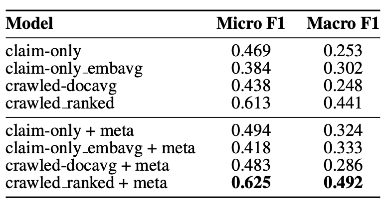
The authors calculate the Micro as well as Macro F1, then mean average results over all domains. The evidence-based claim veracity prediction models outperform claim-only veracity by a large margin. Also, crawled ranked is the best performing model in terms of Micro F1 and Macro F1, meaning that the model captures that not every piece of evidence is equally important, and can be utilised for veracity prediction.
To further explore the other variations of the model, check out the link below to the paper where the authors have explained in detail the other variations on the test set.
The authors conclude that the best performing model is the crawled ranked + meta. They also observed that longer claims are harder to classify correctly, and that claims with a high direct token overlap with evidence pages lead to a high evidence ranking.
Also when it comes to frequently occurring tags and entities, very general tags such as ‘government-and-politics’ or ‘tax’ that do not give away much, frequently co-occur with incorrect predictions. Whereas more specific tags such as ‘brisbane-4000’ or ‘hong-kong’ tend to co-occur with correct predictions.
Similar trends are observed for bigrams. This means that the model has an easy time succeeding for instances where the claims are short, where specific topics tend to co-occur with certain veracities, and where evidence documents are highly informative. Instances with longer, more complex claims where evidence is ambiguous remain challenging.